
Multiple Testing
- Table of Contents
I. Goals
Large-scale approaches have enabled routine tracking of the entire mRNA complement of a cell, genome-wide methylation patterns and the ability to enumerate DNA sequence alterations across the genome. Software tools have been developed whose to unearth recurrent themes within the data relevant to the biological context at hand. Invariably the power of these tools rests upon statistical procedures in order to filter through the data and sort the search results.
The broad reach of these approaches presents challenges not previously encountered in the laboratory. In particular, errors associated with testing any particular observable aspect of biology will be amplified when many such tests are performed. In statistical terms, each testing procedure is referred to as a hypothesis test and performing many tests simultaneously is referred to as multiple testing or multiple comparison. Multiple testing arises enrichment analyses, which draw upon databases of annotated sets of genes with shared themes and determine if there is ‘enrichment’ or ‘depletion’ in the experimentally derived gene list following perturbation entails performing tests across many gene sets increases the chance of mistaking noise as true signals.
This goal of this section is to introduce concepts related to quantifying and controlling errors in multiple testing. By the end of this section you should:
- Be familiar with the conditions in which multiple testing can arise
- Understand what a Type I error and false discovery are
- Be familiar with multiple control procedures
- Be familiar with the Bonferroni control of family-wise error rate
- Be familiar with Benjamini-Hochberg control of false discovery rates
II. Hypothesis testing errors
For better or worse, hypothesis testing as it is known today represents a gatekeeper for much of the knowledge appearing in scientific publications. A considered review of hypothesis testing is beyond the scope of this primer and we refer the reader elsewhere (Whitley 2002a). Below we provide an intuitive example that introduces the various concepts we will need for a more rigorous description of error control in section III.
Example 1: A coin flip
To illustrate errors incurred in hypothesis testing, suppose we wish to assess whether a five cent coin is fair. Fairness here is defined as an equal probability of heads and tails after a toss. Our hypothesis test involves an experiment (i.e. trial) whereby 20 identically minted nickels are tossed and the number of heads counted. We take the a priori position corresponding to the null hypothesis: The nickels are fair. The null hypothesis would be put into doubt if we observed trials where the number of heads was larger (or smaller) than some predefined threshold that we considered reasonable.
Let us pause to more deeply consider our hypothesis testing strategy. We have no notion of how many heads an unfair coin might generate. Thus, rather than trying to ascertain the unknown distribution of heads for some unfair nickel, we stick to what we do know: The probability distribution under the null hypothesis for a fair nickel. We then take our experimental results and compare them to this null hypothesis distribution and look for discrepancies.
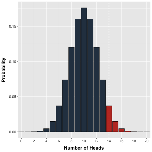
Conveniently, we can use the binomial distribution to model the exact probability of observing any possible number of heads (0 to 20) in a single test where 20 fair nickels are flipped (Figure 1).
plot of chunk unnamed-chunk-1
Figure 1. Probability distribution for the number of heads. The binomial probability distribution models the number of heads in a single test where 20 fair coins are tossed. Each coin has equal probability of being heads or tails. The vertical line demarcates our arbitrary decision threshold beyond which results would be labelled 'significant'.
In an attempt to standardize our decision making, we arbitrarily set a threshold of doubt: Observing 14 or more heads in a test will cause us to label that test as ‘significant’ and worthy of further consideration. In modern hypothesis testing terms, we would ‘reject’ the null hypothesis beyond this threshold in favour of some alternative, which in this case would be that the coin was unfair. Note that in principle we should set a lower threshold in the case that the coin is unfairly weighted towards tails but omit this for simplicity.
Recall that the calculations underlying the distribution in Figure 1 assumes an equal probability of heads and tails. Thus, if we flipped 20 coins we should observe 14 or more heads with a probability equal to the area of the bars to the right of the threshold in Figure 1. In other words, our decision threshold enables us to calculate a priori the probability of an erroneous rejection. In statistical terms, the probability bounded by our a priori decision threshold is denoted or the significance level and is the probability of making an error of type I. The probability of observing a given experimental result or anything more extreme is denoted the p-value. It is worth emphasizing that the significance level is chosen prior to the experiment whereas the p-value is obtained after an experiment, calculated from the experimental data.
Multiple testing correction methods attempt to control or at least quantify the flood of type I errors that arise when multiple hypothesis are performed simultaneously
Definition The p-value is the probability of observing a result more extreme than that observed given the null hypothesis is true.
Definition The significance level () is the maximum fraction of replications of an experiment that will yield a p-value smaller than when the null hypothesis is true.
Definition A type I error is the incorrect rejection of a true null hypothesis.
Definition A type II error is the incorrect failure to reject a false null hypothesis.
Typically, type I errors are considered more harmful than type II errors where one fails to reject a false null hypothesis. This is because type I errors are associated with discoveries that are scientifically more interesting and worthy of further time and consideration. In hypothesis tests, researchers bound the probability of making a type I error by , which represents an acceptable but nevertheless arbitrary level of risk. Problems arise however, when researchers perform not one but many hypothesis tests.
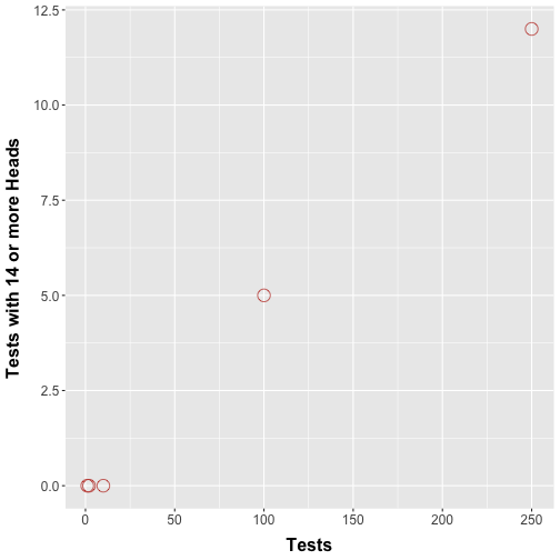
Consider an extension of our nickel flipping protocol whereby multiple trials are performed and a hypothesis test is performed for each trial. In an alternative setup, we could have some of our friends each perform our nickel flipping trial once, each performing their own hypothesis test. How many type I errors would we encounter? Figure 2 shows a simulation where we repeatedly perform coin flip experiments as before.
plot of chunk unnamed-chunk-2
Figure 2. Number of tests where more than 14 heads are observed. Simulations showing the number of times more than 14 heads were counted in an individual test when we performed 1, 2, 10, 100, and 250 simultaneous tests.
Figure 2 should show that with increasing number of tests we see trials with 14 or more heads. This makes intuitive sense: Performing more tests boosts the chances that we are going to see rare events, purely by chance. Technically speaking, buying more lottery tickets does in fact increase the chances of a win (however slightly). This means that the errors start to pile up.
Example 2: Pathway analyses
Multiple testing commonly arises in the statistical procedures underlying several pathway analysis software tools. In this guide, we provide a primer on Gene Set Enrichment Analysis.
Gene Set Enrichment Analysis derives p-values associated with an enrichment score which reflects the degree to which a gene set is overrepresented at the top or bottom of a ranked list of genes. The nominal p-value estimates the statistical significance of the enrichment score for a single gene set. However, evaluating multiple gene sets requires correction for gene set size and multiple testing.
When does multiple testing apply?
Defining the family of hypotheses
In general, sources of multiplicity arise in cases where one considers using the same data to assess more than one:
- Outcome
- Treatment
- Time point
- Group
There are cases where the applicability of multiple testing may be less clear:
- Multiple research groups work on the same problem and only those successful ones publish
- One researcher tests differential expression of 1 000 genes while a thousand different researchers each test 1 of a possible 1 000 genes
- One researcher performs 20 tests versus another performing 20 tests then an additional 80 tests for a total of 100
In these cases identical data sets are achieved in more than one way but the particular statistical procedure used could result in different claims regarding significance. A convention that has been proposed is that the collection or family of hypotheses that should be considered for correction are those tested in support of a finding in a single publication (Goeman 2014). For a family of hypotheses, it is meaningful to take into account some combined measure of error.
The severity of errors
The use of microarrays, enrichment analyses or other large-scale approaches are most often performed under the auspices of exploratory investigations. In such cases, the results are typically used as a first step upon which to justify more detailed investigations to corroborate or validate any significant results. The penalty for being wrong in such multiple testing scenarios is minor assuming the time and effort required to dismiss it is minimal or if claims that extend directly from such a result are conservative.
On the other hand, there are numerous examples were errors can have profound negative consequences. Consider a clinical test applied to determine the presence of HIV infection or any other life-threatening affliction that might require immediate and potentially injurious medical intervention. Control for any errors in testing is important for those patients tested.
The take home message is that there is no substitute for considered and careful thought on the part of researchers who must interpret experimental results in the context of their wider understanding of the field.
The concept that the scientific worker can regard himself as an inert item in a vast co-operative concern working according to accepted rules, is encouraged by directing attention away from his duty to form correct scientific conclusions, to summarize them and to communicate them to his scientific colleagues, and by stressing his supposed duty mechanically to make a succession of automatic ‘decisions’…The idea that this responsibility can be delegated to a giant computer programmed with Decision Functions belongs to a phantasy of circles rather remote from scientific research.
-R. A. Fisher (Goodman 1998)
III. Multiple testing control
The introductory section provides an intuitive feel for the errors associated with multiple testing. In this section our goal is to put those concepts on more rigorous footing and examine some perspectives on error control.
Type I errors increase with the number of tests
Consider a family of independent hypothesis tests. Recall that the significance level represents the probability of making a type I error in a single test. What is the probability of at least one error in tests?
Note that in the last equation as grows the term decreases and so the probability of making at least one error increases. This represents the mathematical basis for the increase probability of type I errors in multiple comparison procedures.
A common way to summarize the possible outcomes of multiple hypothesis tests is in table form (Table 1): The total number of hypothesis tests is ; Rows enumerate the number of true () and false () null hypotheses; Columns enumerate those decisions on the part of the researcher to reject the null hypothesis and thereby declare it significant () or declare non-significant ().
Table 1. Multiple hypothesis testing summary
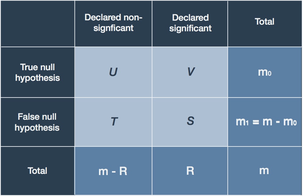
Of particular interest are the (unknown) number of true null hypotheses that are erroneously declared significant (). These are precisely the type I errors that can increase in multiple testing scenarios and the major focus of error control procedures. Below we detail two different perspectives on error control.
IV. Controlling the Family-Wise Error Rate (FWER)
Definition The family-wise error rate (FWER) is the probability of at least one (1 or more) type I error
The Bonferroni Correction
The most intuitive way to control for the FWER is to make the significance level lower as the number of tests increase. Ensuring that the FWER is maintained at across independent tests
is achieved by setting the significance level to .
Proof:
Fix the significance level at . Suppose that each independent test generates a p-value and define
Caveats, concerns, and objections
The Bonferroni correction is a very strict form of type I error control in the sense that it controls for the probability of even a single erroneous rejection of the null hypothesis (i.e. ). One practical argument against this form of correction is that it is overly conservative and impinges upon statistical power (Whitley 2002b).
Definition The statistical power of a test is the probability of rejecting a null hypothesis when the alternative is true
Indeed our discussion above would indicate that large-scale experiments are exploratory in nature and that we should be assured that testing errors are of minor consequence. We could accept more potential errors as a reasonable trade-off for identifying more significant genes. There are many other arguments made over the past few decades against using such control procedures, some of which border on the philosophical (Goodman 1998, Savitz 1995). Some even have gone as far as to call for the abandonment of correction procedures altogether (Rothman 1990). At least two arguments are relevant to the context of multiple testing involving large-scale experimental data.
1. The composite “universal” null hypothesis is irrelevant
The origin of the Bonferroni correction is predicated on the universal hypothesis that only purely random processes govern all the variability of all the observations in hand. The omnibus alternative hypothesis is that some associations are present in the data. Rejection of the null hypothesis amounts to a statement merely that at least one of the assumptions underlying the null hypothesis is invalid, however, it does not specify exactly what aspect.
Concretely, testing a multitude of genes for differential expression in treatment and control cells on a microarray could be grounds for Bonferroni correction. However, rejecting the composite null hypothesis that purely random processes governs expression of all genes represented on the array is not very interesting. Rather, researchers are more interested in which genes or subsets demonstrate these non-random expression patterns following treatment.
2. Penalty for peeking and ‘p hacking’
This argument boils down to the argument: Why should one independent test result impact the outcome of another?
Imagine a situation in which 20 tests are performed using the Bonferroni correction with and each one is deemed ‘significant’ with each having . For fun, we perform 80 more tests with the same p-value, but now none are significant since now our . This disturbing result is referred to as the ‘penalty for peeking’.
Alternatively, ‘p-hacking’ is the process of creatively organizing data sets in such a fashion such that the p-values remain below the significance threshold. For example, imagine we perform 100 tests and each results in a . A Bonferroni-adjusted significance level is meaning none of the latter results are deemed significant. Suppose that we break these 100 tests into 5 groups of 20 and publish each group separately. In this case the significance level is and in all cases the tests are significant.
V. Controlling the false discovery rate (FDR)
Let us revisit the set of null hypotheses declared significant as shown in the right-hand columns of Table 1. Figure 3 is a variation on the Venn diagram showing the intersection of those hypotheses declared significant () with the true () and false () null hypotheses.
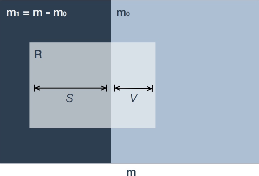
Figure 3. Depiction of false discoveries. Variable names are as in Table 1. The m hypotheses consist of true (m0) and false (m1=m-m0) null hypotheses. In multiple hypothesis testing procedures a fraction of these hypotheses are declared significant (R, shaded light grey) and are termed 'discoveries'. The subset of true null hypotheses are termed 'false discoveries' (V) in contrast to 'true discoveries' (S).
In an exploratory analysis, we are happy to sacrifice are strict control on type I errors for a wider net of discovery. This is the underlying rationale behind the second control procedure.
Benjamini-Hochberg control
A landmark paper by Yoav Benjamini and Yosef Hochberg (Benjamini 1995) rationalized an alternative view of the errors associated with multiple testing:
In this work we suggest a new point of view on the problem of multiplicity. In many multiplicity problems the number of erroneous rejections should be taken into account and not only the question of whether any error was made. Yet, at the same time, the seriousness of the loss incurred by erroneous rejections is inversely related to the number of hypotheses rejected. From this point of view, a desirable error rate to control may be the expected proportion of errors among the rejected hypotheses, which we term the false discovery rate (FDR).
Definition The false discovery proportion () is the proportion of false discoveries among the rejected null hypotheses.
By convention, if is zero then so is . We will only be able to observe - the number of rejected hypotheses - and will have no direct knowledge of random variables and . This subtlety motivates the attempt to control the expected value of .
Definition The false discovery rate (FDR) is the expected value of the false discovery proportion.
The Benjamini-Hochberg procedure
In practice, deriving a set of rejected hypotheses is rather simple. Consider testing independent hypotheses from the associated p-values .
- Sort the p-values in ascending order.
- Here the notation indicates the order statistic. In this case, the ordered p-values correspond to the ordered null hypotheses
-
Set as the largest index for which
-
Then reject the significant hypotheses
-
A sketch(y) proof
Here, we provide an intuitive explanation for the choice of the BH procedure bound.
Consider testing independent null hypotheses from the associated p-values where . Let be the p-values corresponding to the true null hypotheses indexed by the set .
Then the overall goal is to determine the largest cut-off so that the expected value of is bound by
For large , suppose that the number of false discoveries
The largest cut-off will actually be one of our p-values. In this case the number of rejections will simply be its corresponding index
Since will not be known, choose the larger option and find the largest index so that
Proof
Theorem 1 The Benjamini-Hochberg (BH) procedure controls the FDR at for independent test statistics and any distribution of false null hypothesis.
Proof of Theorem 1 The theorem follows from Lemma 1 whose proof is added as Appendix A at the conclusion of this section.
Lemma 1 Suppose there are independent p-values corresponding to the true null hypotheses and are the p-values (as random variables) corresponding to the false null hypotheses. Suppose that the p-values for the false null hypotheses take on the realized values . Then the BH multiple testing procedure described above satisfies the inequality
Proof of Lemma 1. This is provided as Appendix A.
From Lemma 1, if we integrate the inequality we can state
and the FDR is thus bounded.
Two properties of FDR
Let us note two important properties of FDR in relation to FWER. First, consider the case where all the null hypotheses are true. Then , and which means that any discovery is a false discovery. By convention, if then we set otherwise .
This last term is precisely the expression for FWER. This means that when all null hypotheses are true, FDR implies control of FWER. You will often see this referred to as control in the weak sense which is another way of referring to the case only when all null hypotheses are true.
Second, consider the case where only a fraction of the null hypotheses are true. Then and if then . The indicator function that takes the value 1 if there is at least one false rejection, will never be less than Q, that is . Now, take expectations
The key here is to note that the expected value of an indicator function is the probability of the event in the indicator
This implies that and so FWER provides an upper bound to the FDR. When these error rates are quite different as in the case where is large, the stringency is lower and a gain in power can be expected.
Example of BH procedure
To illustrate the BH procedure we adapt a trivial example presented by Glickman et al. (Glickman 2014). Suppose a researcher performs an experiments examining differential expression of 10 genes in response to treatment relative to control. Ten corresponding p-values result, one for each test: . The researcher decides to bound the FDR at 5% (). Table 2 summarizes the ordered p-values and corresponding BH procedure calculations.
Table 2. Example BH calculations
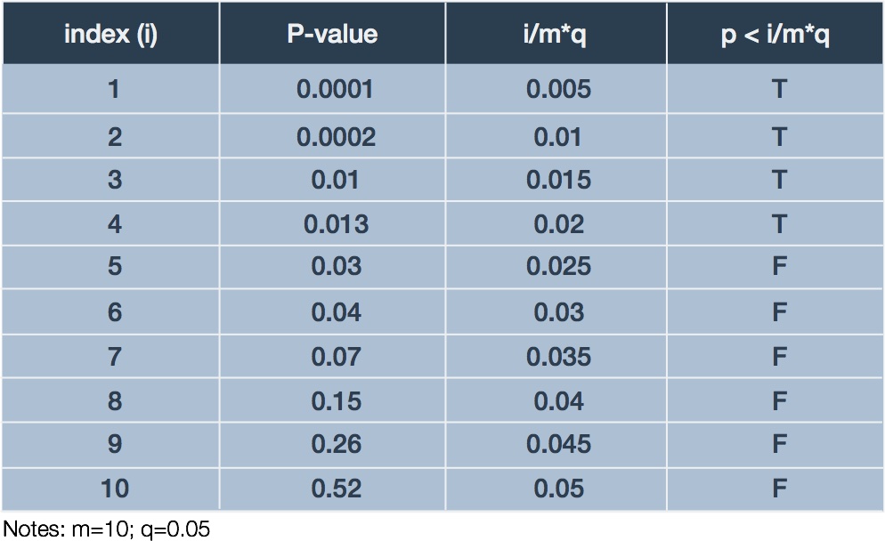
In this case, we examine the final column for the largest case in which which happens in the fourth row. Thus, we declare the genes corresponding to the first four p-values significant with respect to differential expression. Since our we would expect, on average, at most 5% of our discoveries to be mistaken, which in our case is nil.
Practical implications of BH compared to Bonferroni correction
The BH procedure overcomes some of the caveats associated with FWER control procedures.
The “universal” null hypothesis. Control of FWER was predicated upon testing the universal null hypothesis that purely random processes accounts for the data variation. In contrast, the BH approach focuses on those individual tests that are to be declared significant among the set of discoveries .
Penalty for peeking The BH procedure can accommodate the so-called “penalty for peeking” where variations in the number of tests performed alters the number of significant hypotheses. Consider an example where 20 tests are performed with ; The same p-value is derived in an additional 80 tests. In a Bonferroni correction the significance levels are and for 20 and 100 tests, respectively, rendering the latter insignificant. In contrast, the BH procedure is “scalable” as a function of varying numbers of tests: In the case where we require largest such that
All hypotheses will be significant if we can find such a relation to hold for . This is true for such that .
Caveats and limitations
Since the original publication of the BH procedure in 1995, there have been a number of discussion regarding the conditions and limitations surrounding the use of the method for genomics data. In particular, the assumption of independence between tests is unlikely to hold in large-scale genomic measurements. We leave it to the reader to explore more deeply the various discussions surrounding the use of BH or its variants (Goeman 2014).
Appendix A: Proof of Lemma 1
We intend on proving Lemma 1 that underlies the BH procedure for control of the FDR. The proof is adapted from the original publication by Benjamini and Hochberg (Benjamini 1995) with variant notation and diagrams for clarification purposes. We provide some notation and restate the lemma followed by the proof.
Notation
- Null hypotheses:
- Ordered null hypotheses: .
- P-values corresponding to null hypotheses: .
- Ordered P-values corresponding to null hypotheses: .
- Ordered P-values corresponding to true null hypotheses:
- Ordered P-values corresponding to false null hypotheses:
The lemma
Lemma 1 Suppose there are independent p-values corresponding to the true null hypotheses and are the p-values (as random variables) corresponding to the false null hypotheses. Suppose that the p-values for the false null hypotheses take on the realized values . Then the BH multiple testing procedure satisfies the inequality
We proceed using proof by induction. First we provide a proof for the base case . Second, we assume Lemma 1 holds for and go on to show that this holds for .
-
Asides
-
There are a few not so obvious details that we will need along the way. We present these as a set of numbered ‘asides’ that we will refer back to.
1. Distribution of true null hypothesis p-values
The true null hypotheses are associated with p-values that are distributed according to a standard uniform distribution, that is, . The proof of this follows.
Let be a p-value that is a random variable with realization . Likewise let be a test statistic with realization . As before, our null hypothesis is . The formal definition of a p-value is the probability of obtaining a test statistic at least as extreme as the one observed assuming the null hypothesis is true.
Let’s rearrange this.
The last term on the right is just the definition of the cumulative distribution function (cdf) where the subscript denotes the null hypothesis .
If the cdf is monotonic increasing then
The last two results allow us to say that
This means that which happens when .
2. Distribution of the largest order statistic
Suppose that are independent variates, each with cdf . Let for denote the cdf of the order statistic . Then the cdf of the largest order statistic is given by
Thus the corresponding probability mass function is
In the particular case that the cdf is for a standard uniform distribution then this simplifies to
Base case
Suppose that there is a single null hypothesis .
Case 1: .
Since then there are no true null hypotheses and so no opportunity for false rejections , thus . So Lemma 1 holds for any sensible .
Case 2: .
Since then there is a single true null hypothesis (). This could be accepted or rejected .
Induction
Assume Lemma 1 holds for and go on to show that this holds for .
Case 1: .
Since then there are no true null hypotheses and so no opportunity for false rejections , thus . So Lemma 1 holds for any sensible .
Case 2: .
Define as the largest index for the p-values corresponding to the false null hypotheses satisfying
Define as the value on the right side of the inequality at .
Moving forward, we will condition the Lemma 1 inequality on the largest p-value for the true null hypotheses by integrating over all possible values . Note that we’ve omitted the parentheses for order statistics with the true and false null hypothesis p-values. We’ll break the integral into two using as the division point. The first integral will be straightforward while the second will require a little more nuance. The sum of the two sub-integrals will support Lemma 1 as valid for .
Condition on the largest p-value for the true null hypotheses and split the integral on .
The first integral
In the case of the first integral . It is obvious that all p-values corresponding to the true null hypotheses are less than , that is . By the BH-procedure this means that all true null hypotheses are rejected regardless of order. Also, we know that from the definition of , there will be total hypotheses that are rejected (i.e. the numerator). We can express these statements mathematically.
Substitute this back into the first integral.
Finally let’s extract a and substitute it with its definition.
The second integral
Let us remind ourselves what we wish to evaluate.
The next part of the proof relies on a description of p-values and indices but is often described in a very compact fashion. Keeping track of everything can outstrip intuition, so we pause to reflect on a schematic of the ordered false null hypothesis p-values and relevant indices (Figure 4).

Figure 4. Schematic of p-values and indices. Shown are the p-values ordered in ascending value from left to right corresponding to the false null hypotheses (z). Indices j0 and m1 for true null hypotheses are as described in main text. Blue segment represents region where z' can lie. Green demarcates regions larger than z' where p-values corresponding to hypotheses (true or false) that will not be rejected lie.
Let us define the set of p-values that may be subject to rejection, that is, smaller than . Another way to look at this is to define the set of p-values that will not be rejected, that is, larger than .
Consider the set of possible values for defined by the criteria where . In Figure 4 this would correspond to the half-open set of intervals to the right of . If we set , then this same region includes the set of false null hypothesis p-values with indices . We need to consider one more region defined by . In Figure 4 this is the green segment to the right of .
Let us discuss the regions we just described that are larger than . By the BH procedure, these bound p-values for true and false null hypotheses that will not be rejected. Thus, we will not reject neither the true null hypothesis corresponding to nor any of the false null hypotheses corresponding to .
So what is left over in terms of null hypotheses? First we have the set of true null hypotheses less the largest giving a total of . Second we have the set of false null hypotheses excluding the ones we just described, that is, for a total of . This means that there are null hypotheses subject to rejection. Let us provide some updated notation to describe this subset.
If we combine and order just this subset of null hypotheses, then according to the BH procedure any given null hypothesis will be rejected if there is a such that for which
Now comes some massaging of the notation which may seem complicated but has a purpose: We wish to use the induction assumption on the expectation inside the second integral but we will need to somehow rid ourselves of the pesky term. This motivates the definition of transformed variables for the true and false null hypotheses.
Convince yourself that the are ordered statistics of a set of independent random variables while correspond to the false null hypotheses subject to . Also convince yourself that for
In other words, the false discovery proportion of at level is equivalent to testing at .
Now we are ready to tackle the expectation inside the integral.
Let us now place this result inside the original integral.
Let’s now add the results of the two half integrals and .
Thus, Lemma 1 holds for the base case and by the induction hypothesis all . Since we have shown that Lemma 1 holds for , by induction we claim that Lemma 1 holds for all positive integers and the proof is complete.
References
- Benjamini Y and Hochberg Y. Controlling the False Discovery Rate: A Practical and Powerful Approach to Multiple Testing. Roy. Stat. Soc., v57(1) pp289-300, 1995.
- Glickman ME et al. False Discovery rate control is a recommended alternative to Bonferroni-type adjustments in health studies. Journal of Clinical Epidemiology, v67, pp850-857, 2014.
- Goeman JJ and Solari A. Multiple hypothesis testing in genomics. Stat. Med., 33(11) pp1946-1978, 2014.
- Goodman SN. Multiple Comparisons, Explained. Amer. J. Epid., v147(9) pp807-812, 1998.
- Rothman KJ. No Adjustments Are Needed for Multiple Comparisons. Epidemiology, v1(1) pp. 43-46, 1990.
- Savitz DA and Oshlan AF. Multiple Comparisons and Related Issues in the Interpretation of Epidemiologic Data. Amer. J. Epid., v142(9) pp904 -908, 1995.
- Whitley E and Ball J. Statistics review 3: Hypothesis testing and P values. Critical Care, v6(3) pp. 222-225, 2002a.
- Whitley E and Ball J. Statistics review 4: Sample size calculations. Critical Care, v6(4) pp. 335-341, 2002b.